MOHID Water
Particle tracking transport
Lagrangian transport models are very useful to simulate localized processes with sharp gradients:
- Submarine outfalls;
- Phytoplankton blooms;
- Sediment erosion due to dredging works;
- Hydrodynamic calibration;
- Oil dispersion;
- Hazardous and Noxious Substances (HNS);
- Fish larvae dispersion;
- Exchanges between different areas in a estuary;
- Exchanges between the deep ocean and the continental shelf;
- Etc...
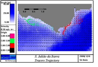
MOHID Lagrangian module uses the concept of tracer. The most important property of a tracer is its position (x,y,z). For a physicist a tracer can be a water mass, for a geologist it can be a sediment particle or a group of sediment particles and for a chemist it can be a molecule or a group of molecules.
A biologist can spot phytoplankton cells in a tracer (at the bottom of the food chain) as well as a shark (at the top of the food chain), which means that a model of this kind can simulate a wide spectrum of processes.
The movement of the tracers can be influenced by the velocity field from the hydrodynamic module, by the wind from the surface module, by the spreading velocity from oil dispersion module and by random velocity.
At the current stage the model is able to simulate oil dispersion, water quality evolution and sediment transport.
To simulate oil dispersion the Lagrangian module interacts with the oil dispersion module, to simulate the water quality evolution the Lagrangian module uses the feature of the water quality module. Sediment transport can be associated directly to the tracers using the concept of settling velocity.
Another feature of the Lagrangian transport model is the ability to calculate residence times. This can be very useful when studying the exchange of water masses in bays or estuaries.
Numerical Characteristics
Main characteristics | |
|---|---|
| Spatial Interpolation | Bilinear horizontally and linear vertically |
| Particle movement | Particle movement can the sum of the follow effects:
|
| Flow turbulence | Random walk based in the turbulent mixing length (constant or turbulence model) and turbulent velocity standard deviation (Allen, 1982a) |
| Land mapping |
|
| Flow and water properties input |
|
| Particles emission | Set of origins In each origin particles can be emitted:
|
| Particles monitoring |
|
| Output |
|
0D coupling | |
|---|---|
| Faecal indicator mortality |
|
| Sediments | Sedimentation velocity imposed or function of D50 Bottom erosion and deposition critical stress |
| Water quality | Water quality modules of MOHID |
| Oil spill |
|
| Hazardous and Noxious Substances (HNS) |
|
| Buoyancy jet model or MOHID Jet |
|
| Renewal and residence time |
|
| Fish larvae |
|
References
aAllen C.M. Numerical simulation of contaminant dispersion in estuary flows. Proceedings of the Royal Society of London A: Mathematical, Physical and Engineering Sciences. 1982; 381(1780): 179-194. doi: 10.1098/rspa.1982.0064
bMOHIDJET Technical Manual (2003). Available for download here
cMOHID Fish larvae manual (2012). Available for download here